Divergent Pathways: Tracking Cryptosporidium’s Host Adaptation

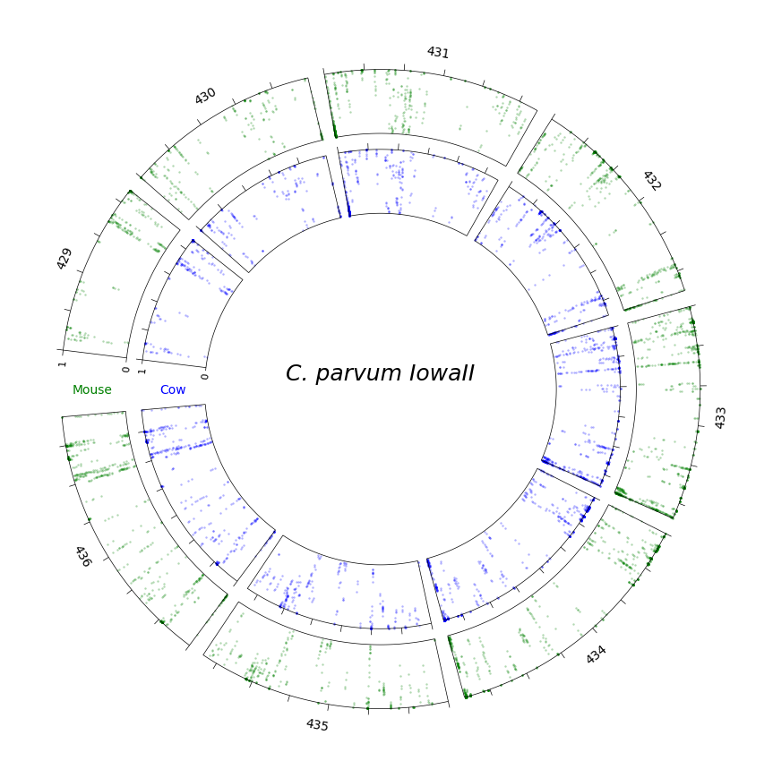
data=pd.read_csv('../data/allele_frequencies.tsv',sep='\t')
make_circos_plot(data)

The Origin: Strain M4

Our journey begins with a single infected mouse (M4), harboring a Cryptosporidium strain that would become the progenitor of two distinct evolutionary paths. This initial host served as the critical branching point for our experimental design.

From this single origin, the parasite’s story split into two parallel narratives:

🐭 The Murine Passage 🐭

In this pathway, Cryptosporidium continued its journey through a series of mouse hosts, adapting to the murine environment through sequential passages:

M4 → M5 → M6 → M7

Each passage potentially allowed the parasite to optimize its survival and reproductive strategies within these genetically similar mammalian hosts.

🐄 The Bovine Passage 🐄

Simultaneously, we challenged the adaptability of the same initial strain by introducing it to an entirely different mammalian lineage - neonatal calves:

M4 → C1 → C2 → C3

This cross-species transmission forced the parasite to navigate a dramatically different physiological environment, potentially driving rapid adaptation.

🧬 Specialized Variant Calling Strategy 🧬

To fully capture the variability of the Cryptosporidium population in mouse M4 we implemented a customized variant calling pipeline:

┌────────────────────────────────┐
│ FREEBAYES VARIANT CALLING      │
├────────────────────────────────┤
│ • Ploidy = 1                   │
│ • --pooled-continuous option   │
└────────────────────────────────┘

Why This Approach Matters?

Beyond Binary Detection: > Traditional presence/absence variant calling would have flattened the rich complexity of our samples, obscuring the very phenomenon we aimed to study. Tipycally variant call in Cryptosporidium is performed with ploidy 2. We belive this is suboptimal as it might filter out variant with more than 2 alleles.
Quantitative Insight: > By focusing on allele frequencies rather than simple variant calls, will allow us to track subtle shifts in population genetics across hosts.

Variant Analysis: Filtering Strategy

Our approach employed a strategic sequence of filtering steps, each addressing specific aspects of data quality:

┌─────────────────────────────────────┐
│ THREE-TIER FILTERING STRATEGY       │
├─────────────────────────────────────┤
│ 1. Quality-based Filtering          │
│ 2. Read Depth Optimization          │
│ 3. Variant Type Selection           │
└─────────────────────────────────────┘

filter_variants()

======================================
Starting Variant Filtering Process
======================================
Total variants before filtering: 15901
Stage 1: QUAL filtering: 14087 Variants removed and 1814 variants left
Stage 2: FORMAT/DP filtering, DP >= 30 & DP <= 150: 355 Variants removed and 1459 variants left
Stage 3: After keeping SNPs and indels: 203 Variants removed and 1256 variants left

Pipline notes

Stage 1: Quality-Based Filtering

# Eliminate low confidence variant calls
bcftools filter -e 'QUAL < 30' "$INPUT_VCF" -o "$QUAL_FILTERED_VCF"

Rationale: The QUAL score represents the statistical confidence in each variant call. By establishing a minimum threshold of 30: - We eliminated variants likely to be sequencing errors - Retained variants with a 99.9% probability of being genuine

Stage 2: Read Depth Optimization

# Balance between coverage requirements and anomalous amplification
bcftools view -i 'FMT/DP >= 30 & FMT/DP <= 150' "$QUAL_FILTERED_VCF" -o "$DP_FILTERED_VCF"

Rationale: Read depth optimization addressed two critical concerns: - Lower bound (DP ≥ 30): Ensured sufficient read coverage - Upper bound (DP ≤ 150): Protected against false positives from regions with anomalous read pileups which often indicate repetitive elements

Stage 3: Variant Type Selection

# Focus on  variation subset
bcftools view -v snps,indels "$DP_FILTERED_VCF" -o "$SNP_FILTERED_VCF"

Rationale: This final step ensured our analysis focused exclusively on:

Single nucleotide polymorphisms (SNPs)
Small insertions and deletions (indels)

From Raw Variants to Biological Insights 📊 with Pandas 🐼

Leveraging the robust capabilities of Python’s pandas library transformed our genetic data into a powerhouse of actionable insights.

┌─────────────────────────────────────────────────────┐
│ DATA TRANSFORMATION PIPELINE                        │
├─────────────────────────────────────────────────────┤
│ 1. Load filtered VCF file                           │
│ 2. Remove ambiguous reference calls (REF = 'N')     │
│ 3. Restructure for for computing frequency          │
└─────────────────────────────────────────────────────┘

vcf_file = "../data/filtered_final.vcf"  
df_vcf = read_vcf(vcf_file)
print(f'step 1: {df_vcf.shape}')
df_vcf=df_vcf[(df_vcf['REF']!='N')]
print(f'step 2: {df_vcf.shape}')

step 1: (1256, 16)
step 2: (945, 16)

df_vcf.head()

	#CHROM	POS	ID	REF	ALT	QUAL	FILTER	INFO	FORMAT	M7	M5	M4	M6	C3	C2	C1
0	CM000429	60867	.	TAAAAAAAAAAGATAT	TAAAAAAAAAAAGATTT,TAAAAAAAAAAAGATAT,TAAAAAAAAA...	10088.400	PASS	AB=0,0,0;ABP=0,0,0;AC=0,7,0;AF=0,1,0;AN=7;AO=1...	GT:GQ:DP:AD:RO:QR:AO:QA:GL	2:138:82:9,2,67,2:9:296:2,67,2:24,2218,68:-172...	2:138:46:3,2,35,1:3:100:2,35,1:24,1116,34:-91....	2:138:69:4,4,59,1:4:132:4,59,1:48,1980,34:-166...	2:138:82:14,2,62,1:14:461:2,62,1:24,2092,26:-1...	2:138:57:5,1,45,1:5:163:1,45,1:12,1492,34:-119...	2:138:69:1,0,60,4:1:34:0,60,4:0,1966,136:-173....	2:138:62:4,1,50,4:4:130:1,50,4:12,1678,128:-13...
1	CM000429	60889	.	ACCCCACT	ACCCCCACT	11705.800	PASS	AB=0;ABP=0;AC=7;AF=1;AN=7;AO=435;CIGAR=1M1I7M;...	GT:GQ:DP:AD:RO:QR:AO:QA:GL	1:137:90:9,81:9:295:81:2686:-215.126,0	1:137:53:1,50:1:34:50:1596:-140.656,0	1:137:70:2,66:2:68:66:2184:-190.372,0	1:137:82:11,70:11:359:70:2241:-169.324,0	1:137:45:5,40:5:169:40:1237:-96.064,0	1:137:68:1,66:1:31:66:2174:-192.923,0	1:137:69:4,62:4:126:62:2002:-168.787,0
2	CM000429	76625	.	A	G	265.872	PASS	AB=0;ABP=0;AC=1;AF=0.142857;AN=7;AO=248;CIGAR=...	GT:GQ:DP:AD:RO:QR:AO:QA:GL	0:131:104:76,28:76:2560:28:952:0,-144.672	0:131:80:52,28:52:1738:28:930:0,-72.6994	0:131:84:50,34:50:1596:34:1156:0,-39.5691	0:131:89:61,28:61:2066:28:944:0,-100.949	1:131:83:36,47:36:1216:47:1598:-34.3706,0	0:131:112:78,34:78:2630:34:1126:0,-135.322	0:131:112:63,49:63:2126:49:1658:0,-42.1062
3	CM000429	82019	.	A	T	8192.190	PASS	AB=0;ABP=0;AC=7;AF=1;AN=7;AO=410;CIGAR=1X;DP=5...	GT:GQ:DP:AD:RO:QR:AO:QA:GL	1:160:98:9,89:9:306:89:2994:-241.841,0	1:160:51:15,36:15:510:36:1186:-60.8115,0	1:160:86:19,67:19:638:67:2240:-144.133,0	1:160:90:15,75:15:488:75:2488:-179.952,0	1:160:70:26,44:26:862:44:1472:-54.8869,0	1:160:81:31,50:31:1046:50:1662:-55.4182,0	1:160:71:22,49:22:748:49:1666:-82.5935,0
4	CM000429	82192	.	G	A	6765.840	PASS	AB=0;ABP=0;AC=6;AF=0.857143;AN=7;AO=398;CIGAR=...	GT:GQ:DP:AD:RO:QR:AO:QA:GL	1:134:104:11,93:11:374:93:3124:-247.418,0	1:134:67:20,47:20:658:47:1598:-84.5836,0	1:134:75:25,50:25:842:50:1692:-76.4771,0	1:134:102:26,76:26:846:76:2568:-154.943,0	0:0:53:28,25:28:944:25:850:0,-8.45503	1:134:92:35,57:35:1190:57:1938:-67.2984,0	1:134:83:33,50:33:1084:50:1692:-54.7114,0

📝 From VCF Fields to counting reads for each allele

┌─────────────────────────────────────────────────────────┐
│ ALLELE FREQUENCY CALCULATION COMPONENTS                 │
├─────────────────────────────────────────────────────────┤
│ RO: Reference Allele Observation count                  │
│ AO: Alternate Allele Observation count                  │
│ DP: Total Read Depth at position                        │
│                                                         │
│ Allele Frequency = AO / DP                              │
└─────────────────────────────────────────────────────────┘

df_allele_counts = expand_multiallelic_variants(df_vcf)
df_allele_counts.to_csv("../data/allele_counts_expanded.tsv", sep="\t", index=False)
print("✅ Extracted and expanded allele counts saved to allele_counts_expanded.tsv")

✅ Extracted and expanded allele counts saved to allele_counts_expanded.tsv

df_allele_counts.head()

	#CHROM	POS	REF	ALT	INFO_TYPE	RO_M7	DP_M7	AO_M7	RO_M5	DP_M5	...	AO_M6	RO_C3	DP_C3	AO_C3	RO_C2	DP_C2	AO_C2	RO_C1	DP_C1	AO_C1
0	CM000429	60867	TAAAAAAAAAAGATAT	TAAAAAAAAAAAGATTT	complex	9	82	2	3	46	...	2	5	57	1	1	69	0	4	62	1
1	CM000429	60867	TAAAAAAAAAAGATAT	TAAAAAAAAAAAGATAT	ins	9	82	67	3	46	...	62	5	57	45	1	69	60	4	62	50
2	CM000429	60867	TAAAAAAAAAAGATAT	TAAAAAAAAAAAAGATAT	ins	9	82	2	3	46	...	1	5	57	1	1	69	4	4	62	4
3	CM000429	60889	ACCCCACT	ACCCCCACT	ins	9	90	81	1	53	...	70	5	45	40	1	68	66	4	69	62
4	CM000429	76625	A	G	snp	76	104	28	52	80	...	28	36	83	47	78	112	34	63	112	49

5 rows × 26 columns

📝 Keep variants where one of the call as at least 5 supporting reads

shell we also remove complex? yes for now

print(df_allele_counts.shape)
df_allele_counts = df_allele_counts[
df_allele_counts[[n for n in df_allele_counts.columns if n.startswith('AO')]].max(axis=1)>=5]
df_allele_counts = df_allele_counts[df_allele_counts['INFO_TYPE']!='complex']
print(df_allele_counts.shape)

(1937, 26)
(1121, 26)

df_af = compute_frequencies(df_allele_counts)
df_af.to_csv("../data/allele_frequencies.tsv", sep="\t", index=False)
print("✅ Allele frequencies saved to allele_frequencies.tsv")

✅ Allele frequencies saved to allele_frequencies.tsv

df_af.head()

	#CHROM	POS	REF	ALT	AF_M7	AF_M5	AF_M4	AF_M6	AF_C3	AF_C2	AF_C1
1	CM000429	60867	TAAAAAAAAAAGATAT	TAAAAAAAAAAAGATAT	0.817073	0.760870	0.855072	0.756098	0.789474	0.869565	0.806452
3	CM000429	60889	ACCCCACT	ACCCCCACT	0.900000	0.943396	0.942857	0.853659	0.888889	0.970588	0.898551
4	CM000429	76625	A	G	0.269231	0.350000	0.404762	0.314607	0.566265	0.303571	0.437500
5	CM000429	82019	A	T	0.908163	0.705882	0.779070	0.833333	0.628571	0.617284	0.690141
6	CM000429	82192	G	A	0.894231	0.701493	0.666667	0.745098	0.471698	0.619565	0.602410

🔍 Frequency Distribution Analysis

With our extracted allele frequencies in hand, we could now explore how these frequencies were distributed across our samples

fig,ax=plt.subplots(figsize=(8,4))
data=pd.read_csv('../data/allele_frequencies.tsv',sep='\t')
tmp = pd.Series(data.iloc[:,4:].values.flatten())
tmp.name='All Samples'
tmp.plot(kind='hist',histtype='step',bins=50,ax=ax,linewidth=1)
ax.set_xlabel('Alternate Allele Frequency')
ax.set_ylabel('Counts')
mod_hist_legend(ax)
clean_axes(ax)
plt.show()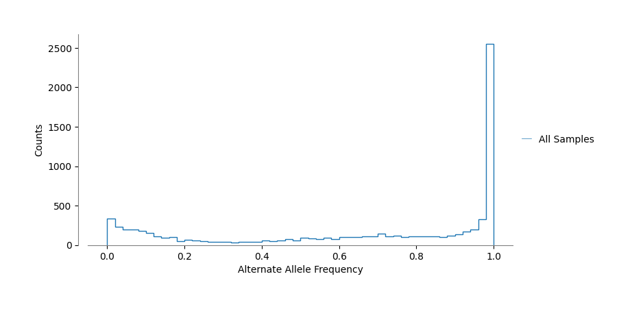

Expected in a population: Frequencies clustered at extremes (0 or 1)

“with also allele frequencies deviating from the expected 0/1 pattern”

🔬 Focusing on Single Nucleotide Variants

To gain deeper insight into the evolutionary dynamics of our Cryptosporidium populations, we narrowed our analysis to focus specifically on Single Nucleotide Variants (SNVs).

┌─────────────────────────────────────────────────────────┐
│ SNV CLUSTERING WORKFLOW                                 │
├─────────────────────────────────────────────────────────┤
│ 1. Filter dataset to retain only SNVs                   │    
│ 2. Normalize frequencies (divide by max frequency)      │
│ 4. Include only variants with >30% frequency            │
│    difference between any two samples                   │
│ 5. Perform hierarchical clustering                      │
│ 6. Visualize dendrogram                                 │
└─────────────────────────────────────────────────────────┘

Prepare data and visualize SNVs frequencies

from ProjectUtility.core import clean_axes
import numpy as np
fig,axes =plt.subplots(ncols=4,nrows=2,figsize=(12,4))
axes=axes.flatten()
for i, col in enumerate(['AF_M7', 'AF_M5', 'AF_M6', 'AF_M4','AF_C3', 'AF_C2', 'AF_C1']):
    #col = 'AF_'+run
    run = col.split('_')[1]
    tmp = data.copy()
    tmp = tmp[(tmp['REF'].str.len()==1) & (tmp['ALT'].str.len()==1)]
    tmp = tmp[['#CHROM', 'POS', col]]
    tmp = tmp[tmp[col]>0]
    title = col#mapping.get(run,run)
    plot_chromosomal_af_values2(tmp, axes[i])
    axes[i].set_title(col.split('_')[1])   
    axes[i].set_ylabel('Frequency',fontsize=12)
    axes[i].set_xlabel('Chromosome', labelpad=10,fontsize=12)
        #clean_axes(axes[new_i])
axes[-1].set_axis_off()
plt.tight_layout()
plt.savefig('../data/Chromosome_Frequency.png')
plt.savefig('../data/Chromosome_Frequency.svg')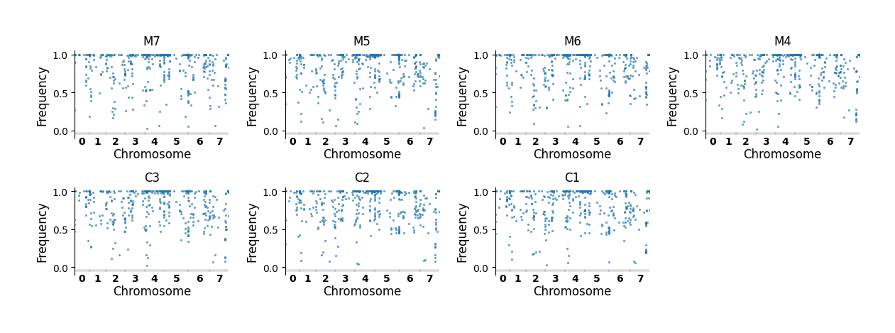

Prepare data and visualize upset plot

from upsetplot import UpSet
from upsetplot import from_contents
import matplotlib.pyplot as plt

data=pd.read_csv('../data/allele_frequencies.tsv',sep='\t')
print(f'step 1 starting variants: {data.shape}')
data=data[(data['ALT'].str.len()==1)]
print(f'step 2 only snv variants: {data.shape}')

clustering_data = data[['#CHROM','POS','AF_M7', 'AF_M5', 'AF_M6', 'AF_M4','AF_C3', 'AF_C2', 'AF_C1']]
clustering_data=clustering_data.set_index(['#CHROM','POS'])
clustering_data.columns = ['M7', 'M5', 'M6', 'M4','C3', 'C2', 'C1']
print(clustering_data.shape)
clustering_data=clustering_data.reset_index(drop=True)
upset_data = (clustering_data>0).reset_index()
upset_data=upset_data.set_index(['M7', 'M5', 'M6', 'M4','C3', 'C2', 'C1'])
upset_data.columns=['variant']
#upset_data.head()

ax_dict = UpSet(upset_data, 
                subset_size="count",
                sort_by='input',
                sort_categories_by='input',
                show_counts=True,
               ).plot()
nvariants = upset_data.shape[0]
ax_dict['intersections'].set_title(f'N variants: {nvariants}',y=1.1)
plt.savefig('../data/Upset_all.png')
plt.savefig('../data/Upset_all.svg')
plt.show()

step 1 starting variants: (1121, 11)
step 2 only snv variants: (511, 11)
(511, 7)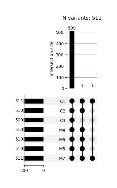

'2.3.0'

Visualizing Selected SNVs Frequencies

data=pd.read_csv('../data/allele_frequencies.tsv',sep='\t')
print(f'step 1 starting variants: {data.shape}')
data=data[(data['ALT'].str.len()==1)]
print(f'step 2 only snv variants: {data.shape}')

clustering_data = data[['#CHROM','POS','AF_M7', 'AF_M5', 'AF_M6', 'AF_M4','AF_C3', 'AF_C2', 'AF_C1']]
clustering_data=clustering_data.set_index(['#CHROM','POS'])
clustering_data = clustering_data.divide(clustering_data.max(axis=1),axis=0)
clustering_max=clustering_data.max(axis=1)
clustering_min=clustering_data.min(axis=1)
clustering_data = clustering_data[(clustering_max-clustering_min)>0.3]
clustering_data.columns = ['M7', 'M5', 'M6', 'M4','C3', 'C2', 'C1']
clustering_data=clustering_data.reset_index(drop=True)
print('selected variants:', clustering_data.shape)
g = sns.clustermap(clustering_data,cmap='Blues',figsize=(6,6),cbar_pos=(0.02, 0.82, 0.04, 0.15))
g.fig.axes[2].set_yticks([])
plt.savefig('../data/Allele_Frequency_SNVs.svg')
plt.savefig('../data/Allele_Frequency_SNVs.png')

step 1 starting variants: (1121, 11)
step 2 only snv variants: (511, 11)
selected variants: (129, 7)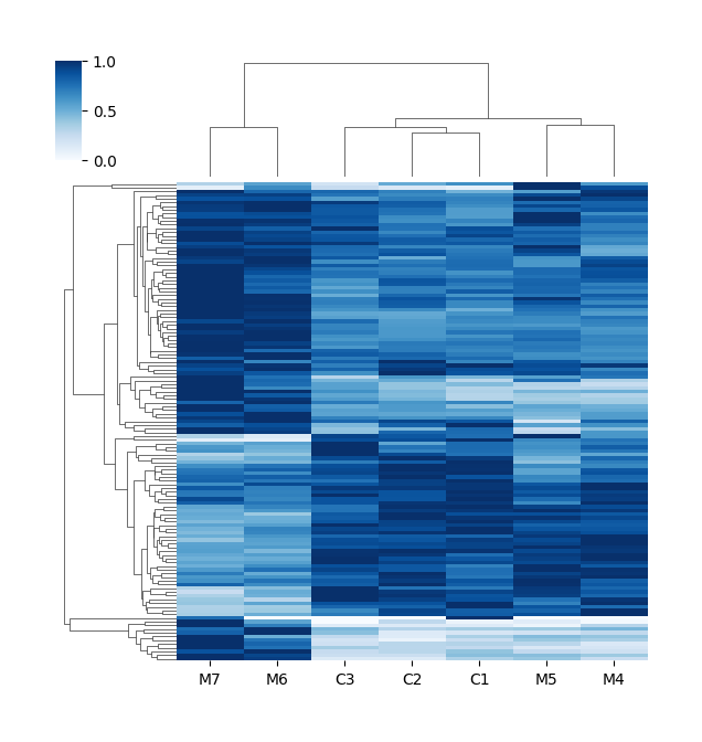

🧬 Variant Observations

No novel variant identified: > “Using our filtering strategy we could not detect SNV unique to one sample, but only frequency variations of the initial variant pool.”

🧬 Distinct Evolutionary Trajectories Revealed

The hierarchical clustering dendrogram revealed several patterns:

Clear Host-Species Separation: > “The clustering segregated bovine and murine samples, suggesting host specific pressure on the Cryptosporidium population.”
Temporal Evolution in Murine Hosts: > “The murine samples displayed a clear temporal progression, with M6 and M7 clustering distinctly from the earlier passages (M4-M5).”
Similarity Between Early Murine and Bovine Samples: > “The three bovine samples (C1-C3) showed greater similarity to the early murine passages (M4-M5) than to the later murine passages (M6-M7). Bovine adaptation might be slower to kick in.”
Caveats: > “We might be overinterpret results, the variation in frequency might be due to fluctuations/sampling in the population used for the M6 infection”

Genome-Wide Distribution: Mapping Variants Across the Cryptosporidium Genome

🔍 Taking a Broader Perspective

Having explored the dynamics SNVs through clustering analysis, we step back to examine the holistic picture of where variants (SNVs and INDELs) are distributed across the Cryptosporidium genome.

data=pd.read_csv('../data/allele_frequencies.tsv',sep='\t')
make_circos_plot(data)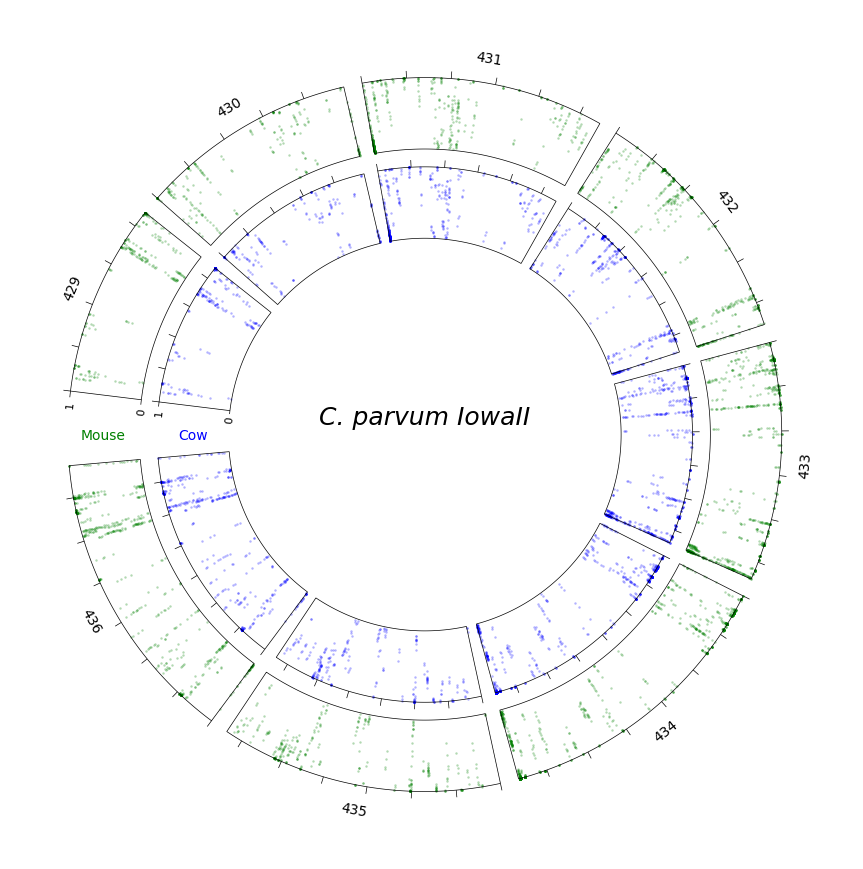

🧬 Genomic Distribution Patterns

The circular genome plot revealed several striking patterns:

“The distribution of variants across the Cryptosporidium genome is strikingly non-random, with clear hotspots of both SNVs and INDELs congregating in specific genomic regions other then close to the telomers as alredy observed in other study”

🧬 Expanding Comparative Analysis

We plan to compare our samples with other environmental and outbreak-related Cryptosporidium genome sequencing projects.

Reproducibility and Availability

The complete analysis pipeline is available as a Python package in our GitHub repository

Installation

pip install git+https://github.com/mtinti/cryptosporidium_host_adaptation.git

Dependencies

This pipeline was developed and tested with: - samtools (Version: 1.21) - bcftools (Version: 1.21)

Interactive Analysis

For interactive exploration and reproducibility, we provide Jupyter notebooks accessible through MyBinder. > The computational environment includes all necessary dependencies pre-configured.